Showing posts with label LabView. Show all posts

Saturday, November 10, 2012

Home-made cyclic voltammetry system, part III

Earlier I have written two post about making your own cyclic-voltammetry measurement system, in that concept a combination of PXI-system and homebuilt electronics were used. In this post I make a completely new cyclic-voltammetry system and with a different approach, that is by using a source measurement unit (SMU).

Background

The reason for this is that I fortunately have a few 100 volts PXI-4132, from National Instruments, source measurement unit (SMU) cards left over and the specifications of these cards are very good, 2 watt of power up to 100 volts and current measurement resolution in picoampere range.
A source measurement unit is sort of an advanced power supply but with the difference that it can also sink power, that is drain a battery for example. On top of that the source measurement unit can operate as both a current source or a voltage source and if the card can do both this when sinking and sourcing power one say it has four-quadrant capabilities. Last due to the technic of a source measurement unit one automatically measure the current/voltage when sourcing voltage/current.

Tutorial: Cyclic-voltammetry

Cyclic-voltammetry is used when one wants to analyse electrode-material, and/or some electro-chemical process. This is done by using three electrodes. Two of them are used for the electro-chemical process and the electric current goes through these two. If one monitors the potential over these two electrodes as one need to do in order to make a IV-graph, or if you repeat the IV-measurement in cycles a CV-graph, data will look strange, se figure 1:blue curve, what one wants is the red-curve in the same figure. The blue curve is from three consecutive voltage cycles so one also wants the blue lines to overlap better.
Figur 1, two CV curves from the SMU unit, blue is two-probe configuration and red is three. The blue curve shows instability problems. All electrodes were copper-wires.

This problem, they say, is due to the current that goes through the electrodes making potential unstable, however there is a solution to this and that is were the third electrode comes in.
The third electrode is connected in such a way (high-ohmic thing) so that a minimum of electric current will pass through it and therefore measuring the potential against this electrode thereby reducing instability problem, that is the red curve of figure 1.
The one of the two current handling electrodes you use for potential measurement against the reference electrode is called the working electrode, the other current handling electrode is called counter electrode. If you make experiments on the electrode itself, the working electrode, is the one you use and the counter electrode is then used only for suppling/collecting current from the electrolyte. The counter electrode must be made in such a way so that it dosent interfere with the process for example limiting the current flow due to too smal electrode surface area.

The last thing to write about this is that the material of the reference electrode is free to be chosen. This because the reference electrode do not handle electric current and therefore is not directly involved in the electrochemical process. In the red curve of figure 1 a copper wire were used as reference electrode. One can instead use a more fancier electrode, like the Ag/AgCl type, specifically constructed for this task.

Figur 2, An standard Ag/AgCl electrode.

Because this Ag/AgCl electrode is a standard electrode, and its properties is well-known one can compare measurements from different experiments. Silver-Chloride is also light sensitive so one shall probably not keep this one out in daylight too long, I think.

Method and Results

Sourcing voltage while measuring the current as done in cyclic voltammetery sound like a most suitable task for a source measurement unit. The problem is the reference electrode, i.e. how to connect it.
Figure 3, the PXI-4132 SMU card and were to plug in the electrodes.

The PXI-4132 source measurement unit card has sensing outputs, that means the card can do four-probe measurement and when doing so, the card do not measure the sourced voltage at the source itself but rather at the ends of a cables connected to the sense connectors. Figure 3 and 4 shows how to connect the cables to the card. The sense option on the card is made in such way so when used it dosent drain current from the point that you want to measure and that is exactly what we want for the reference electrode, just plug it in. You measure voltage between the working electrode and the reference electrode so therefore you also need to connect the left over sensing output to the working electrode or as in the figure, a short yellow cable between the two outputs.

Figure 4, the connector and cables used together with the card (left) and the copper wires used as electrodes (right).

I have tested the concept preliminary by doing some cyclic voltammetry on a acetic/acetate solution with two copper wires as working and counter electrodes and a Ag/AgCl electrode as reference, figure 5 red curve. Figure 6 shows a similar run, but made on tap-water and here I wanted to check different sweep-rate speeds and repeatability.
Figure 5, CV-graph of acetic/acetate solution at 20mV/s sweep rate. Two copper-wire electrodes used together with a Ag/AgCl reference electrode (red) and with copper reference electrode (blue). The middle peak in red curve that is missing in blue curve I do not know what it is.
Figure 6, CV-graph of tap-water at different sweep rates, the dots and the red curve corresponds to two separate measurements but with same parameters and the good overlap indicates good performance and stability of the system.

Discussion

The results seems promising but I have yet to try a more advanced experiment to test its performance level. Tap-water or Sodium bicarbonate from the kitchen as used above is perhaps not so advanced, but it shows the princip that the system is operational.

The drawback of the source measurement unit card is that it is not so fast, for cyclic voltammetry the speed is fine but if you want to do frequency analysis like Nyqvist plots the speed will not be enough so that is not an options for this system. A few thousands of samples per seconds is the limit of the card.
On the other hand, the flexibility of the source measurement unit is of great use: want galvanostatic mode?, no problem, just configure the card as current sourcing instead as voltage source. Current or voltage limits can also just as easily be set. This particular source measurement unit card can handle up to 100 volts, and that is interesting, cause it allows me to do charge/discharge experiments on more voltage demanding task and the high resolution and picoampere capabilities allows monitoring of very low constant-charge current levels, that is 200 nA as lowest level. These two capabilities is good for example capacitor experiments.

Integration of curve or other calculations can be included in the labView code. Table below shows how I made the output log file to look like, five simple columns in a txt file were the two last ones are integration values of curent and voltage.


#Volt/s:   1m Smp/cycle: 1000 numb of cycles:   5
#---------------------------------------------------------------
#Time(s),   Current(A), Potential(V),  Int.   I(J),   Int. U(Vs)
   0.003    1.99645E-5   -1.47711E-2    8,12327E-5   -1,81089E-2
   0.022    1.99672E-5   -1.98860E-2    3,99317E-5   -3,46570E-2
   0.059    1.99711E-5   -2.27894E-2    2,01308E-5   -2,29280E-2
   0.095    1.99686E-5   -2.42637E-2    2,00491E-5   -2,43554E-2


Here is the link to the LabView code I wrote for this, the ZIP-file is a snapshot from May this year so there might be some trash/experimental code inside it as well, beware.

Conclusion

Using a SMU card (PXI-4132), seems to work very well for cyclic voltammetry measurements, flexibility is good and might be of great use. Speed is low so Nyquist measurements is not possible. I think I will report back on this topic when I done some more advanced experiment with this setup.

Tuesday, July 19, 2011

Home-made cyclic voltammetry system, part II

This post is an update to the previous post: homemade-cyclic-voltammetry-system.html.

Background
In the last post I described how to build a cyclic-voltammetry-system using LabVIEW and some PXI-system components. Some unsolved problems was periodic noise in the CV measurements, and that the Nyquist method was not completely developed, here you find an update on the subject.

CV measurements
The periodic noise I had last time in the CV-graphs was from settling time problems when measuring the voltage-outputs from the operational amplifiers with the digital acquisition card. By doing the reading directly before the next output voltage value (the voltage sweep) is written this noise was completely removed. (previously measurements were done directly after the new voltage value was written.

Figure 1, CV measurement test, now the periodic noise is removed.

Nyquist measurement
Now everything works properly, and the software program has been completed. Both the Fourier method with white noise and the frequency sweep method now works. I found out that for larger capacitance measurements, i.e. lower frequencies dependency, the sweep method works better.
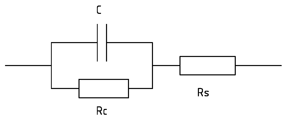
Figure 2, shows some basic Nyquist test experiment of 1uF capacitor in parallel with 1kOhm resistor and all this in series with 100 Ohm.

Fuse installed
To protect the circuit I decided to install a fuse.
Figure 3, I now also included a 50mA fuse to protect the circuit. 

Well, that was the update, now this case is closed. The next post will be a little bit more interesting.
Here are two links for the LabVIEW 2010 code for the CV and Nyquist program.

There is now a continuation on this topic, Home-made-cyclic-voltammetry-system III.

Monday, December 6, 2010

Home-made cyclic voltammetry system

Today I will report on a side-topic, an home-made cyclic voltammetry system  (most of my posts are usually about electron microscopy).


Background
A potentiostat is a device capable of producing IV curve measurements that shows hysteresis effects due to various chemical reactions, the potentiostat does this by keeping the applied potential at the conter electrode at a fixed level in relation to the reference electrode during the measuring of the outgoing electrical current in the working electrode. The conter electrode is can be made of platinum, while the reference electrode is more advanced in its construction, and are usually bought as is, this to certify that several different measurements can be compared to a known electrode. The working electrode is the one you want to measure. 
The idea for building this potentiostat is the need for measurements on fabricated capacitors and electrodes. For the electrodes this device could be used to caracterize the electrode functionality in an electrochemical cell and for the capacitors, electrical characterization can be made and especially the AC-dependency is an important property to measure. 
Currently we don not posses  the proper instrumentation for this.


Method
The idea is to use the National Instruments PXI measurement system with some simple electric circuitry to be able to make cyclic voltammetry system.  We are also interested in conducting AC-dependent measurement such as Nyquist plots.


I read the book by Allen J. Bard, Electrochemical methods, Wiley, from the year 1980 it contained some basic electronic circuitry drawings for building a potentiostat. 


The device is made around a simple circuit with just a few operational amplifiers. Building a bipotentiostat is no more thing than adding one more amplifier, so I decided to do that as well. The bipotentiostat is used when you use a rotating ring disk electrode, at the moment this is not something we directly need, but perhaps in a near future. The connector block SCB-68 of the PXI system features 5V power supply, to drive the amplifiers I choose to include a DCP020515D, switching voltage IC that supplies ±15V out of 5V. As regarding the operational amplifiers I used CA3140E standard MOSFET amplifier, mainly because I have some left overs from earlier experiments.
 
Figure 1, (left) electrical drawing of the components used, color coding matches the photo (right) of the SCB-68 connector block with the operational amplifiers (four small IC) and the switching IC (the big one).

Results
For the reference electrode I found a Ag/AgCl type in the lab. The conter electrode is made up of wiring a 0.25 mm platinum wire around a glass rod. The working electrode is a DSA-electrode prototype, I will not write anymore onto this as the topic is just to verify the operational status of the built potentiostat. Se figur 2, for the experimental setup.

Figur 2, (left) the setup of the electrochemical cell, and a detailed photo (right), the black square electrode in the front beaker is the working electrode, the conter electrode is the platinum wire on the glass rod and, the reference Ag/AgCl electrode is seen in the other beaker at the back thats in turn is connected to the cell by the bent pipet. 

The LabView software code is is an algoritm that sends out a ramp up and down signal for the voltage sweep while taking measurements of the current from the working electrode. As can be seen in the screen dump most basic functions of cyclic voltammetry can be controlled, i.e sweep rate, scan limits, number of cycles etc.
Figure 3, screen dump of the LabView program in operation.


The plot below shows the basic cyclic voltammetry result. The curve is partly what one can expect from this DSA electrode, the curve shows some basic hysteresis effects, however it also contains unknown peaks around the intervall 0.35V-0.40V which I at the moment do not know the meaning of. The noise that can be seen around the curve is also of strange origin and seems partly periodic, and repetitively and in coherence for each cycle sweep.  
Figure 4, The cyclic voltammetry plot of the test run.

The AC measurement method, I have at this moment just tried out very momentarily. The first goal is to produce a Nyquist plot of a simple electronic setup of a resistor in series with a capacitor and a resistor, se figure 5.


Figur 5, (top) the simple electrical setup for the Nyquist measurements. (bottom) the corresponding Nyquist plot, the offset of the half cirlce from the vertical axis is related to the series resistance, while the diameter of the half circle corresponds to the capacitors parallell resistance, the height of the circle is linked to the capacitance.

I conducted this test by introducing white noise into the setup and thereafter Fourier transform the measured result to produce the Nyquist plot, as seen in figure 5. This approach is easier and quicker than the regular sweeping of the frequency method, especially if you can do it in software. 

The produced Nyquist plot shows the right shape for the electrical setup being tested but unfortunately it is not correct to the values and at least 30% error can be observed. Later I will try the more basic frequency sweeping method instead.

Conclusion
This homemade potentiostat seems to work partly, cause it shows some basic cyclic voltammetry results, however there still remains some unsolved question regarding peaks and noise as seen in the plots. The AC methods have not been tested yet to any larger extent.


There is now an update to this post in the home-made-cyclic-voltammetry-system, part II post.

Friday, October 8, 2010

Optical temperature measurement in-situ TEM

I promised to report back on the latest ongoing project, i.e. temperature measurement in-situ transmission electron microscopy (TEM).

Background
At our lab we usually do a lot of in-situ TEM experiment with special types of sample holders that have a movable probe. The probe is used to contact and characterize nanomaterials and in these experiments most often electrical current is used to probe and heat up the sample. However measurements of the actual temperature induced by this electrical heating is problematic in these types of two-probe setup. We know the input electrical power and can model and estimate the temperature based on this. But dissipation of heating energy in contact resistances make this a rather uncertain method. A direct temperature method would be most useful and by introducing a optical fiber into the system, this is possible for higher temperatures, i.e. above 1000 Kelvin, by measuring the blackbody spectra.


Benefits of putting an optical fiber inside the TEM
One can think of several benefits:


Method
As mention before, we use special types of sample holders. That is modified versions of the Nanofactory Instruments AB, se figure 4, holders. Because these holders already have electrical wiring to control the probe in front of the holder they are easily modified to fit more wiring or as in this case an optical fiber. This project was driven as a two student projet at bachelor university level in which the students modified the holder with the insertion of an optical fiber during a period of ten weeks. Great thanks to these two good students of the Mid Sweden University.


The most obvious problem is how to get the optical fiber inside the vacuum system of the TEM without introducing a leak. We chose to build our solution on an optical fiber patch cord 200um of VIS/NIR type from Edmund Optics. This saved us time as we did not need to assemble the optical SMA contacts that the spectrometer uses.


Most technical details can be seen in the drawing shown below, figure 1, so here I only write some supporting information. The patch cord is held in place by fitting and squeezing  an O-ring tight around the cord with a screw metal plate clamping, se figure 2. This to avoid unwanted tension in the accutal fiber that goes through the sample holder.


Figure 1 (top), the schematic drawing of the modified sample holder with an optical fiber. Figure 2 (left), The backside of the sample holder, here one can se the screw clamping of the fiber patch cord at the top.
Figure 3 (right), the front of the sample holder, here one can se the moving probe (right) used for contacting and heating nano materials. At the top one can se the optical fiber, here with light coming out in the end of it. In front of the fiber is placed a 45 degree angle rod mirror coated with aluminum this to direct the black body radiation from the sample (center of image, oposite to the probe) into the fiber. Figure 4 (bottom), the sample holder in hole. The front to the left and the modified backside of the holder to the right in image. This holder is used in a JEOL-2000fx transmission electron microscope.

Back of sample holder
The fiber patch cord is unwrapped and the fiber is left exposed at the front of the clamping position. Here the fiber is threaded through a rubber-plug and this plug is fixated in a tapered hole, this gives a high vacuum tight seal, some Fomblin grease was used to make things slide more easily. By the way remember that if you instead have an ultra high vacuum system, rubber is not allowed. After the plug the fiber is continuing towards into the front of the sample holder. To assemble this a fishing line was used and threaded from the oposite direction and glued to the top of the fiber to help threading and guiding the fiber through the holder. 

Front of sample holder
The fiber is threaded through and comes out in the front of the sample holder at the side of the probe, se figure 3 and cut with a tweezer-cutter to proper length. First we thought that some fixation device was needed to hold the fiber in place but since the 200um optical fiber is quit stiff this was not needed. We also did not notice any problems with charging due to the e-beam exposure of the fiber.
To direct the light produced by the heated sample into the fiber a mirror was used. We bought a rod mirror of diameter 1mm from Edmund Optics for this purpose, it is aluminum coated so charging by the e-beam would be less problematic.  We also bought a prism but did not use this for the same reason that the beam might charge this uncoated prism, se figure 5. The mirror was glued with electrical conductive glue onto a Pt/Ir stiff wire that was fitted into a metall tube that was in-turn glued to the side of the holder and at the front of the fiber, this to allow for proper adjustment of the mirror so that the radiation from the sample could be directed into the fiber, se figure 3. Light was led through the fiber in the oposite direction, i.e. from the spectrometer side, to make proper alignment of the fiber-mirror-sample system.
Figure 5, rod mirror with aluminum coating and a diameter of 1mm (left) and the prism that was not used  due to believed electric beam charging (right).

Spectrometer
We used a previously bought spectrometer from Edmund Optics for the first tests, it is a relabeled BWTEK CCD-spectrometer of VIS-NIR type. It has sensitivity up to 1000nm wavelength. The sensitivity drops almost linearly from 500nm to 1000nm by 75% which is of course quit bad for blackbody experiments which has it's peaks around 1000nm, but it did well for a first test result as seen figure 6. 

Results
What we did was to heat up, by driving an electrical current through, a sample of Mo6S3I6 nanowires. The sensitivity was not enough to record the blackbody radiation intensity from a single nanowire bundle but only when severals was heated at the same time. The spectrometer gives a curve that resembles quit well a curve from previously measured well defined temperature source of 1300 Kelvin (furnace) so the conclusion is that the samples was heated to the same temperature, se figure 6.
Figure 6 (left), spectrometer data of the first in-situ TEM experiments when a Mo6S3I6 nanowire sample is heated up to 1300 Kelvin, as proven by the calibration curve from a furnace test. Figure 7 (right) CNT 's heated up to almost 2800 Kelvin, compared to a tungsten lamp source spectra, the lamp spectra is somewhat flooded in the detector counts at its peak.

If you know some blackbody radiation, se wikipedia for example, theory you know that the peak of the radiation spectra would be 1000nm for a tungsten lamp at 2800 Kelvin and the peak in our diagram above was found at a shorter wavelength thus indicating an even higher temperature than this. Of course this is not the case thus the observed peak is due to the spectrometers dropping sensitivity for increasing wavelength, one can correct this curve to a known temperature source so it shows the real blackbody curve, however this is not shown as this beyond the topic of this blog post. We also tried heating up carbon nanotubes, here also with severals at the same time but here we achieved a must higher temperature of almost 2800 Kelvin as seen if one compares the data with a tungsten lamp source at 2800 Kelvin, se figure 7. Due to the higher temperature the blackbody intensity is increased dramatically which is beneficial for the detector. Previously we used the maximum integration time of the spectrometer, that is 60s, but here we could lower this to 10s and yet still, half of the maximum count of the detector was achieved.

Conclusion
The method of using an optical fiber patch cord to introduce in-situ temperature measurements in the TEM worked. Blackbody radiation intensity was recorded for a Mo6S3I6 sample heated to a temperature of 1300 Kelvin as well as a carbon nano tube sample heated to 2800 Kelvin. The used spectrometer was not optimum, a better chice would have been a Prime X spectrometer or a Sol 1.7 spectrometer from BWTEK which has a better sensitivity in the range of 800nm to 1200nm. Higher wavelength sensitivity will probably not be needed as blackbody spectra in these wavelength would be of to weak intensity anyway.

Whats next
Currently we are working on making the hole system of this in-situ TEM probing mobile by utilizing a PXI-measurement system from National Instruments.

Good sailing on the sea of knowledge /Dr. Hummelgård

Thursday, July 15, 2010

Digital images from old SEM/STEM detectors and CRT's

Background
The TEM that we have, the Jeol 2000fx is equipped with two extra detectors, one secondary electron detector, i.e. SEM imaging, as well as a STEM detector at the bottom of the microscope.
Because the system are from the 80's the imaging from these detectors is (read "was") accomplished by using photographic film to copy the image shown on the CRT. An extra CRT monitor specifically used for this task is located in a free standing box in which the camera with light sensitiv polaroid film is attached to.

Nowadays, everything is digital, and polaroid imaging is therefore not very user friendly or timesaving. Besides, one of the two CRT's used for setting upp the image to be captured is broke in our system and the other one is almost burned out... -Time to move into the next century of technology.

Electronics
By different means I found out that the ASID panel, i.e the one that controls the scanning of the electron beam during SEM/STEM imaging, has a extra contact hidden behind the backpanel, labeled SG6, figure 1.
Figure 1, After opening the back-panel of the ASID unit the signal generator card (SG) is somewhat exposed as well as the extra contact SG6, used for external scan control.

If one looks at the circuit diagram, figure 2, one can se that the external scan mode is activated by connecting pin 5 of the SG6 to ground. This mode bypass the scan generator function of the ASID panel and allows you to insert your own scan signals at pin 1 and 2 for horisontal and vertical. The signal level happens to be ±10 Volts and this is lucky thus the PXI-6229 card that I use for this task also has this amplitude range limit. To connect to the SG6 I assembled a signal cable from SG6 internally to the front of the ASID, a switch was used to connect pin 5 to ground, and the horisontal and vertical scan signals got two SMB panel connectors, se figure 3.

Figure 2, the circuit diagram, the essential connector pins for external scan mode is marked with red. Click image to enlarge it.

figure 3 There was one free slot on the ASID front-panel that I used for the switch and connectors. (left) the backside of the ready made front-panel and the frontside of it (right).

The detectors each have BNC connector output I just simply detached the regular cables to these ones and connected my own that leads to the same DAQ-card as mentioned above. This electronic setup will results in that the ASID unit will just handle signal conditioning between my DAQ-card and the beam-scan coils, the two (three) CRT's will no longer be needed. The only buttons on the ASID panel in use will be stigmatism correction and detector contrast setting.

LabView
What you want to do is to get LabView to generate two signals, two sawtooth for horisontal and vertical synch signals. I configured this as a single DAQ-task where both are written at the same time to avoid conflicts on the hardware.  During signal generation you also need to collect the detector data, this I configured as a parallel task to one the above. You have one options here and that's to read data faster than you write, this will improve signal noise ratio for you and I made this option as a user "scan speed" selection in the program. I always read data as fast as possible, 200kHz, and depending on what slower scan speed setting one choose, more samples are read for each position on the sample.

You also have another option here and that is to scan one horisontal line then collect the data from the detector or to read the hole image in one sampling. The former gives you ability to handle bigger image sizes, i.e. beyond 512x512 pixels images, because you only need to have one scan line in the DAQ-card buffer each time. The later alternative is of-course much faster. I choose to implement booth, the one-line scan mode for final imaging and the hole-image scan mode for fast preview as this gives you almost 2 frames/s in 128x128 pixels.

As a final option for improving signal to noise ratio I also made integration over several imaging, i.e. adding images together, as an user option.

Results
To test out the new system configuration I inserted a sample of gold-nanoparticles roughly 50nm in diameters, located on a standard TEM grid.
Figure 4, TEM image of gold-nanoparticles (left) and STEM image of the same, but rotated 90° CCV (right).

Figure 5, SEM image of the same sample and region as shown in figure 4, but at slightly lower magnification this time. Resolution is in this quick check seems to be around 50 nm for the SEM imaging mode, but I expect this to improve if one tveek the system to more optimal settings. (the green color is for those of us who misses the green CRT monitor.)
Future work
Due to the in-situ probing that we usually do in our setup we can measure the impact beam current of the sample during SEM scan and make mapping of this as well this is yet to be done and I report on this later.

Tuesday, June 29, 2010

Jeol EM-SHH (heating holder) fix

A sample heating holder
Is a device that makes it possible to heat the TEM-grid during observation inside the TEM. These special holders can usually go up to temperatures beyond 1000°C with make’s it pretty neat to study anealing, crystalisation and other related phenomena for metals or other types of materials.


-The good’s, I acquried an used heating holder of Jeol fabricate and it fits our microscope, the 2000fx that is.

-The bad’s, no manual, no power supply only the actual holder was devliered.

Solution:
1. Use National Instruments PXI system as replacement for the missing power supply unit.
+. This gives a bonus of complete integration to the rest of our system setup, sync with video recording, logging etc.

Some subproblems to consider:
Find out the cable configuration on the back of the holder. These holder’s usually contains a thermocouple (TC) to measure (two wires) the temperature and a filament (another two wires) to heat the sample with. In figure 2 below one sees a photo of the back of the holder, showing the connected wires from the grey cable that goes to the connector that fits in the power supply unit. An ohm meter will give you which wires belong to each other but to find out which pair is the thermocouple and which is the filament one need to measure the resistance temperature dependency of the pairs. I used the PXI system to measure the temperature dependency. In this case it was the RED and WHITE wires. This means that the remaining pair BLACK and GREEN are used for the filament.

I decided to remove the old contact on the heating holder and replace it with a new one of Fischer type.
Figure 1, the Fischer connector (103 type) that was assembled onto the heating holder cable.
To find out what type of TC is being used
I search the Internet and found a paper describing that a similar holder used a thermocouple of PT-PT-RH(13%) combination, R-type that is.

The paper was:
Crystallization of amorphous thin low pressure chemical vapour deposition silicon films' in situ TEM measurement of grain growth rates
J. P. GUILLEMET, B. DE MAUDUIT, B. PIERAGGI, E. CAMPO and E. SCHEID
JOURNAL OF MATERIALS SCIENCE LETTERS 12 (1993) 910-912

I quick test to see if this is also right for my holder was done. I measured the temperature using the R-type configuration of the thermocouple and melted a small piece of Indium metal that I have placed on the TEM grid. According to the temperature reading of the thermocouple, the metal melted at 155°C, table value states 156.6°C for Indium so this is within the error range and the thermocouple is most likely of R-type.
Figure 2, The back side of the heating holder RED, WHITE thermocouple and BLACK, GRREN heating filament.


The thermocouple circuit
Just to mention som technical details about the temperature measurement. I use a PXI system with the National Instrument's PXI-6229 multifunctional M-series DAQ in combination with a SCB-68 connector block. This is a sleek setup for thermocouple measurements, the LabView software has preconfigured scaling for thermocouples, you just select which type you wanna use, and the SCB-68 connector block has built in cold-junction-compensation by utilizing a LM34 temperature sensor. Because the thermocouple is differential you easily get noise built up in the wires, so I soldered a pair of 10kOhm resistors from the thermocouple lines to ground in the connector box. A low-pass filter with cut of frequency of 4 Hz was also assembled in the connector box. For me this setup gave a signal that is stable to sub ±1°C.

The heating filament circuit
The heating of the filament also need's some signal conditioning setup. First a thought of using a power operational amplifier, but I find out that I already got a ULN2003, a driving stage, in my Racco box so that have to do. This drive-stage has seven channels that works similar to a relay, when a channel is activated on the drive-stage, by a digital TTL signal, it connects the signal to be controlled to ground. I configured all seven channels into a parallel resistors net, where the resistors where configured with the following values: 10, 20, 43, 89, 160, 320 and 650 Ohm. So what does this mean: If I activate the 10 Ohm channel I am sinking an high current due to the low resistance (hot filament) and if I activate a high resistance channel (less hot filament), a smaller current will pass to ground. Because all my seven channels goes through the filament and due to the neat chose of resistors (note the factor of 2x increase between each of them) I can control the heating power level of the filament in 255 step using a binary combination of all the channels.

One thing to consider here is that you limit the heating current by using resistors, the driving stage can sink up to 500mA per channel, so this means that you could get up to 2.5 Watts of heat production in your 10 Ohm resistor, so have this in thought when choosing resistors. I choose a power resistor capable of handling 4 Watts for the 10 Ohm resistor channel, and the 20 Ohm resistor a choose two 1 Watts resistors in series. For the rest the power level is less than 0.5 Watts so for those the power levels are not a problem.

The drive stage is supplied externally with a voltage source.

Figure 3, The SCB-68 connector box with the extra electronics assembled. Top left you se the low-pass filter, (the blue capacitor and resistor) used for the thermocouple, below left is the Fischer connector that goes to the heating holder. The Fischer connector was chosen by me because the one that was on the heating holder was of some old model. To the bottom right you se incoming power supply for the ULN2003, drive stage, the IC located in the middle. Below the IC is the parallell resistor net with a high power resistor to the outer most right of them.
Figure 4, I used Multisim to model the electric circuit to see if the heating powers of the resistors were below the maximum specifications of them.  
The result
I configure a PID control in LabView to control the heating of the filament with the measured  temperature as feed back, a simple program that doesn't need to be shown here I think. This program is now linked to my other LabView program so I will get movie and logging capabilities of a heating experiment.

I tested to heat up the filament, as can bee seen in the graph below, the temperature is considerably higher inside the TEM (vacuum) compared to outside were you will also have a cooling effect by the air.
For air 680mA of heating current gives a temperature of 155°C, were inside the TEM this current level will give you a temperature of roughly 800°C.
Figure 5, Measured temperature as function of heating electric current. Resistance curve is the modeled total resistance including the limiting resistors net. Voltage curve is the modeled applied voltage to the connector box. Heating power is the modeled heating power that the filament produces.

Update
The resistors I used earlier in this experiment were very old and after some running time they could not withstand the heat. So I bought new 2 Watts resistors, as seen in the figure 6.

Figure 6, Resistors, right in picture, were replaced with fresh ones of 2 Watt type, except the 4W power resistor that was still ok. The new coaxial cable seen in this picture, compared with the last, is only used in an another type of experiment.