Home-made cyclic voltammetry system, part III

Earlier I have written two post about making your own cyclic-voltammetry measurement system, in that concept a combination of PXI-system and homebuilt electronics were used. In this post I make a completely new cyclic-voltammetry system and with a different approach, that is by using a source measurement unit (SMU).

Background

The reason for this is that I fortunately have a few 100 volts PXI-4132, from National Instruments, source measurement unit (SMU) cards left over and the specifications of these cards are very good, 2 watt of power up to 100 volts and current measurement resolution in picoampere range.
A source measurement unit is sort of an advanced power supply but with the difference that it can also sink power, that is drain a battery for example. On top of that the source measurement unit can operate as both a current source or a voltage source and if the card can do both this when sinking and sourcing power one say it has four-quadrant capabilities. Last due to the technic of a source measurement unit one automatically measure the current/voltage when sourcing voltage/current.

Tutorial: Cyclic-voltammetry

Cyclic-voltammetry is used when one wants to analyse electrode-material, and/or some electro-chemical process. This is done by using three electrodes. Two of them are used for the electro-chemical process and the electric current goes through these two. If one monitors the potential over these two electrodes as one need to do in order to make a IV-graph, or if you repeat the IV-measurement in cycles a CV-graph, data will look strange, se figure 1:blue curve, what one wants is the red-curve in the same figure. The blue curve is from three consecutive voltage cycles so one also wants the blue lines to overlap better.

Figur 1, two CV curves from the SMU unit, blue is two-probe configuration and red is three. The blue curve shows instability problems. All electrodes were copper-wires.

This problem, they say, is due to the current that goes through the electrodes making potential unstable, however there is a solution to this and that is were the third electrode comes in.
The third electrode is connected in such a way (high-ohmic thing) so that a minimum of electric current will pass through it and therefore measuring the potential against this electrode thereby reducing instability problem, that is the red curve of figure 1.
The one of the two current handling electrodes you use for potential measurement against the reference electrode is called the working electrode, the other current handling electrode is called counter electrode. If you make experiments on the electrode itself, the working electrode, is the one you use and the counter electrode is then used only for suppling/collecting current from the electrolyte. The counter electrode must be made in such a way so that it dosent interfere with the process for example limiting the current flow due to too smal electrode surface area.

The last thing to write about this is that the material of the reference electrode is free to be chosen. This because the reference electrode do not handle electric current and therefore is not directly involved in the electrochemical process. In the red curve of figure 1 a copper wire were used as reference electrode. One can instead use a more fancier electrode, like the Ag/AgCl type, specifically constructed for this task.

Figur 2, An standard Ag/AgCl electrode.

Because this Ag/AgCl electrode is a standard electrode, and its properties is well-known one can compare measurements from different experiments. Silver-Chloride is also light sensitive so one shall probably not keep this one out in daylight too long, I think.

Method and Results

Sourcing voltage while measuring the current as done in cyclic voltammetery sound like a most suitable task for a source measurement unit. The problem is the reference electrode, i.e. how to connect it.

Figure 3, the PXI-4132 SMU card and were to plug in the electrodes.

The PXI-4132 source measurement unit card has sensing outputs, that means the card can do four-probe measurement and when doing so, the card do not measure the sourced voltage at the source itself but rather at the ends of a cables connected to the sense connectors. Figure 3 and 4 shows how to connect the cables to the card. The sense option on the card is made in such way so when used it dosent drain current from the point that you want to measure and that is exactly what we want for the reference electrode, just plug it in. You measure voltage between the working electrode and the reference electrode so therefore you also need to connect the left over sensing output to the working electrode or as in the figure, a short yellow cable between the two outputs.

Figure 4, the connector and cables used together with the card (left) and the copper wires used as electrodes (right).

I have tested the concept preliminary by doing some cyclic voltammetry on a acetic/acetate solution with two copper wires as working and counter electrodes and a Ag/AgCl electrode as reference, figure 5 red curve. Figure 6 shows a similar run, but made on tap-water and here I wanted to check different sweep-rate speeds and repeatability.

Figure 5, CV-graph of acetic/acetate solution at 20mV/s sweep rate. Two copper-wire electrodes used together with a Ag/AgCl reference electrode (red) and with copper reference electrode (blue). The middle peak in red curve that is missing in blue curve I do not know what it is.

Figure 6, CV-graph of tap-water at different sweep rates, the dots and the red curve corresponds to two separate measurements but with same parameters and the good overlap indicates good performance and stability of the system.

Discussion

The results seems promising but I have yet to try a more advanced experiment to test its performance level. Tap-water or Sodium bicarbonate from the kitchen as used above is perhaps not so advanced, but it shows the princip that the system is operational.

The drawback of the source measurement unit card is that it is not so fast, for cyclic voltammetry the speed is fine but if you want to do frequency analysis like Nyqvist plots the speed will not be enough so that is not an options for this system. A few thousands of samples per seconds is the limit of the card.
On the other hand, the flexibility of the source measurement unit is of great use: want galvanostatic mode?, no problem, just configure the card as current sourcing instead as voltage source. Current or voltage limits can also just as easily be set. This particular source measurement unit card can handle up to 100 volts, and that is interesting, cause it allows me to do charge/discharge experiments on more voltage demanding task and the high resolution and picoampere capabilities allows monitoring of very low constant-charge current levels, that is 200 nA as lowest level. These two capabilities is good for example capacitor experiments.

Integration of curve or other calculations can be included in the labView code. Table below shows how I made the output log file to look like, five simple columns in a txt file were the two last ones are integration values of curent and voltage.

#Volt/s:   1m Smp/cycle: 1000 numb of cycles:   5

#---------------------------------------------------------------

#Time(s),   Current(A), Potential(V),  Int.   I(J),   Int. U(Vs)

   0.003    1.99645E-5   -1.47711E-2    8,12327E-5   -1,81089E-2

   0.022    1.99672E-5   -1.98860E-2    3,99317E-5   -3,46570E-2

   0.059    1.99711E-5   -2.27894E-2    2,01308E-5   -2,29280E-2

   0.095    1.99686E-5   -2.42637E-2    2,00491E-5   -2,43554E-2

Here is the link to the LabView code I wrote for this, the ZIP-file is a snapshot from May this year so there might be some trash/experimental code inside it as well, beware.

Conclusion

Using a SMU card (PXI-4132), seems to work very well for cyclic voltammetry measurements, flexibility is good and might be of great use. Speed is low so Nyquist measurements is not possible. I think I will report back on this topic when I done some more advanced experiment with this setup.

Home-made cyclic voltammetry system, part II

This post is an update to the previous post: homemade-cyclic-voltammetry-system.html.

Background
In the last post I described how to build a cyclic-voltammetry-system using LabVIEW and some PXI-system components. Some unsolved problems was periodic noise in the CV measurements, and that the Nyquist method was not completely developed, here you find an update on the subject.

CV measurements
The periodic noise I had last time in the CV-graphs was from settling time problems when measuring the voltage-outputs from the operational amplifiers with the digital acquisition card. By doing the reading directly before the next output voltage value (the voltage sweep) is written this noise was completely removed. (previously measurements were done directly after the new voltage value was written.

Figure 1, CV measurement test, now the periodic noise is removed.

Nyquist measurement

Now everything works properly, and the software program has been completed. Both the Fourier method with white noise and the frequency sweep method now works. I found out that for larger capacitance measurements, i.e. lower frequencies dependency, the sweep method works better.

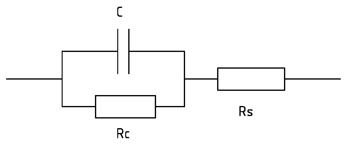
Figure 2, shows some basic Nyquist test experiment of 1uF capacitor in parallel with 1kOhm resistor and all this in series with 100 Ohm.

Fuse installed

To protect the circuit I decided to install a fuse.

Figure 3, I now also included a 50mA fuse to protect the circuit. 

Well, that was the update, now this case is closed. The next post will be a little bit more interesting.

Here are two links for the LabVIEW 2010 code for the CV and Nyquist program.

There is now a continuation on this topic, Home-made-cyclic-voltammetry-system III.

Home-made cyclic voltammetry system

Today I will report on a side-topic, an home-made cyclic voltammetry system  (most of my posts are usually about electron microscopy).


Background
A potentiostat is a device capable of producing IV curve measurements that shows hysteresis effects due to various chemical reactions, the potentiostat does this by keeping the applied potential at the conter electrode at a fixed level in relation to the reference electrode during the measuring of the outgoing electrical current in the working electrode. The conter electrode is can be made of platinum, while the reference electrode is more advanced in its construction, and are usually bought as is, this to certify that several different measurements can be compared to a known electrode. The working electrode is the one you want to measure. 
The idea for building this potentiostat is the need for measurements on fabricated capacitors and electrodes. For the electrodes this device could be used to caracterize the electrode functionality in an electrochemical cell and for the capacitors, electrical characterization can be made and especially the AC-dependency is an important property to measure. 
Currently we don not posses  the proper instrumentation for this.


Method
The idea is to use the National Instruments PXI measurement system with some simple electric circuitry to be able to make cyclic voltammetry system.  We are also interested in conducting AC-dependent measurement such as Nyquist plots.


I read the book by Allen J. Bard, Electrochemical methods, Wiley, from the year 1980 it contained some basic electronic circuitry drawings for building a potentiostat. 


The device is made around a simple circuit with just a few operational amplifiers. Building a bipotentiostat is no more thing than adding one more amplifier, so I decided to do that as well. The bipotentiostat is used when you use a rotating ring disk electrode, at the moment this is not something we directly need, but perhaps in a near future. The connector block SCB-68 of the PXI system features 5V power supply, to drive the amplifiers I choose to include a DCP020515D, switching voltage IC that supplies ±15V out of 5V. As regarding the operational amplifiers I used CA3140E standard MOSFET amplifier, mainly because I have some left overs from earlier experiments.

 

Figure 1, (left) electrical drawing of the components used, color coding matches the photo (right) of the SCB-68 connector block with the operational amplifiers (four small IC) and the switching IC (the big one).

Results

For the reference electrode I found a Ag/AgCl type in the lab. The conter electrode is made up of wiring a 0.25 mm platinum wire around a glass rod. The working electrode is a DSA-electrode prototype, I will not write anymore onto this as the topic is just to verify the operational status of the built potentiostat. Se figur 2, for the experimental setup.

Figur 2, (left) the setup of the electrochemical cell, and a detailed photo (right), the black square electrode in the front beaker is the working electrode, the conter electrode is the platinum wire on the glass rod and, the reference Ag/AgCl electrode is seen in the other beaker at the back thats in turn is connected to the cell by the bent pipet. 

The LabView software code is is an algoritm that sends out a ramp up and down signal for the voltage sweep while taking measurements of the current from the working electrode. As can be seen in the screen dump most basic functions of cyclic voltammetry can be controlled, i.e sweep rate, scan limits, number of cycles etc.

Figure 3, screen dump of the LabView program in operation.

The plot below shows the basic cyclic voltammetry result. The curve is partly what one can expect from this DSA electrode, the curve shows some basic hysteresis effects, however it also contains unknown peaks around the intervall 0.35V-0.40V which I at the moment do not know the meaning of. The noise that can be seen around the curve is also of strange origin and seems partly periodic, and repetitively and in coherence for each cycle sweep.  

Figure 4, The cyclic voltammetry plot of the test run.

The AC measurement method, I have at this moment just tried out very momentarily. The first goal is to produce a Nyquist plot of a simple electronic setup of a resistor in series with a capacitor and a resistor, se figure 5.

Figur 5, (top) the simple electrical setup for the Nyquist measurements. (bottom) the corresponding Nyquist plot, the offset of the half cirlce from the vertical axis is related to the series resistance, while the diameter of the half circle corresponds to the capacitors parallell resistance, the height of the circle is linked to the capacitance.

I conducted this test by introducing white noise into the setup and thereafter Fourier transform the measured result to produce the Nyquist plot, as seen in figure 5. This approach is easier and quicker than the regular sweeping of the frequency method, especially if you can do it in software. 

The produced Nyquist plot shows the right shape for the electrical setup being tested but unfortunately it is not correct to the values and at least 30% error can be observed. Later I will try the more basic frequency sweeping method instead.

Conclusion
This homemade potentiostat seems to work partly, cause it shows some basic cyclic voltammetry results, however there still remains some unsolved question regarding peaks and noise as seen in the plots. The AC methods have not been tested yet to any larger extent.


There is now an update to this post in the home-made-cyclic-voltammetry-system, part II post.

Contact resistance measurement in carbon nano cone

By measuring at several sites along the height of a carbon nano cone, the contact resistance can be calculated. In this experiment we used a cone shaped nano material with a total length/height of 7.59 um, as can be seen in the movie below.

The simple sketch below shows the system setup. At the top left is the gold-probe with the attached carbon nano cone, the sharp needle looking thing and in the bottom right is the opposing movable gold-probe that is used for resistance measurements.


To estimate the contact resistance one need to make a model of the geometry of the cone and it's dependency on resistance, this will give a non-linear curve (for a cone) in a resistance vs length plot. Curve fitting of the model can be made to the data and this determines the resistivity of the material and the unknown contact resistance, and in this case the later is 5.06 kOhm.



Below you can see the calculations for the modeling of the solid cone.

Improvment on meassured variables

By measuring the best known variables, applied bias voltage U, electric current I and the known series resistor with resistance Rs. The unknown variables of the sample, potential drop Up, sample resistance Rs, power in sample Pp was calculated with lesser noise.

$latex U_s=IR_s$
$latex U_p=U-U_s$
$latex R_p=\frac{U}{I}-R_s$
$latex P_p=UI-I^2R_s$

I have remade the plots with this new approach and it clearly shows much better noise-ratio than before. The calulations before were made by using the noisy-value of the measured potential drop over sample.

The sintering image folder at flicker shows you the other plots that were remade.

Details on the sintering process of the nano particles

I have now made some detailed plots on the observed current-jump that occurs when the nano particles fuses together. This was observed for seven of the eight experiments.

In the box archive I have put a data table for the results on the electrical properties. The samples don't have so well defined geometry, but at least they can be aranged unde some basic shapes as wire-, cluster- and grape-shaped. In three cases the need power to sinter the particles was below 1~uW, two cases at 5.9uW and 7.1uW and another two cases at 23.5uW and 34.2uW which is the highest value of them all.

Detail study on the melting of one nanoparticle

In this experiment we manged to study the melting of one single silver nano particle of size 50 nm. What we do is driving a electric current through the sample and continually increasing the power which results in melting of the particles. After the particle have melted a carbon-shell is left behind and the resulting drop in electric resistance is about 800 Ohm.

If one checks the movie from the experiment, one can see that in the beginning of the experiment the same contact particle as mentioned above melts a little with a resulting small decrease in size followed by a resistance increase of 240 Ohm.