Short Guide: Install Python and Gnuplot in Os X

Background

There are two software tools that I always uses:

• Python, programming language, www.python.org
• Gnuplot, plotting software, www.gnuplot.info

However to get this up and running on an Apple Mac with Os X, is not always straightforward. Here I give you a guide of how to set this up on a Mac Os X mountain lion (10.8.2), from a clean install.

The bads:

• The python you got with your Mac Os X is just the main python package, usually, you would like to have some additional packages like numpy or scipy if you does scientific work, as I do.
• For gnuplot, you might want to use the latest functions, or perhaps use animated gif's output then you need to compile gnuplot by your self and you can not use some of the old binaries that are floating around on the Internet. Compile under Os X is usually not so straight forward.
• GCC, the c-compiler, is not included by default in Os X.

The goods:

• Mac os X, has some kind of "unix" back-end, if I am making it short. This means for you an opportunity to use some of the tools from that world, like gnuplot for example. 
• Python is a neat kind of language, and to this date, this is already included in Mac Os X. (python version 2.7.2)
• For the python package's that you usually need, Chris Fonnesbeck, have made a very nice procedure.
• If you know were to look, GCC, can easily be downloaded.
• You have this guide, that you reading know, hopefully that can help you.

This guide is split into two parts: python part I and gnuplot part II. The time consumed for you to do the first part, I estimate to be less than 10 minutes. The second part, however,  takes ruffly one hour of time, and is depending on how much earlier experience you have with the terminal window of your mac. Of-course if you do not need both tools, you can do either part separately, thats up to you.

Part I: 

Install of Python's Extra Packages by Using Chris Fonnesbeck Procedure

1. Open up a new terminal-window in Os X and simply write in one line (copy/paste is easiest):
   sudo curl -o install_superpack.sh https://raw.github.com/fonnesbeck/ScipySuperpack/master/install_superpack.sh
   and the result will looks like this:
   

   
   As noticed you will have to give login password for your computer to make it start downloading the script-file named install_superpack.sh.
2. Now we need to run this script, so write this in the same terminal window:
   sudo sh install_superpack.sh
   
   The script will download and install a bunch of essential packages for python, and this might take some time (<20 min) if you are on a slow connection.
3. That's it now we have the most essential packages installed and we can do some serious work. The packages installed were:
   
   *PyMC is a python module that implements Bayesian statistical models and fitting algorithms, including Markov chain Monte Carlo.
   
   *Statsmodels is a Python package that provides a complement to scipy for statistical computations including descriptive statistics and estimation and inference for statistical models.
   
   *pandas is a Python package providing data structures designed to make working with "relational" or "labeled" data both easy and intuitive for doing practical, real world data analysis in Python.
   
   *IPython: One of Python’s most useful features is its interactive interpreter. The goal of IPython is to create a comprehensive environment for interactive and exploratory computing.
   
   *matplotlib is a python 2D plotting library which produces publication quality figures in a variety of hardcopy formats and interactive environments across platforms.
   
   *SciPy includes modules for statistics, optimization, integration, linear algebra, Fourier transforms, signal and image processing, ODE solvers, and more.
   
   *NumPy is the fundamental package needed for scientific computing with Python. This package contains: a powerful N-dimensional array object, sophisticated (broadcasting) functions, tools for integrating C/C++ and Fortran code, useful linear algebra, Fourier transform, and random number capabilities.
4. We can make a quick test and trying to load some of the modules into python to see if everything went OK. Start python in a terminal windows by simply writing python, then in the python interpreter just started, write import scipy if the >>> prompt just returned back then everything went probably fine. This is how it shall look like if OK:
   
   
   

   

   
   ...and if it was not OK, you will instead see:
   
   

   

Part II: 

Compile and Install of Gnuplot

1. First we need to download the gcc compiler, this is part of the xcode package from apple, but  I do not use xcode, and so I just want the command-line-tools and these can be downloaded just as easily. Firstly go to Apples developer web page,
   
     that is https://developer.apple.com/downloads/.
   
   You will have to login with your apple_id. Search for the dmg-file: "Command Line Tools (OS X Mountain Lion) for X code" and download it, (~110Mb). Install it by open the downloaded file, then click on the package and follow the on-screen instructions.
   
   
   
2. You can test if the gcc was installed properly by open up a terminal window and writing g++, This is how it  shall look like:
   

   
   ...and if it was not installed properly:
   
   

   
3. Now we are ready to download and compile the necessary extra stuff that you need in order to compile gnuplot. Now the tuff part starts. The problem is that if you want to compile gnuplot, you will find out that you need some additional libraries installed in order to do this, and these additional libraries will also require some libraries.... that needs some extra libraries...etc, and so on, so forth. To make it simple for you, I have collected all the extra stuff you need in one download:
   
   you can download it here (these libraries were downloaded Jan-2013).
   
   However I will mention during each step, were you can go to grab the latest versions if you like. The additional stuff required is given in this list below and must be processed in list order, so lets start with, freetype2. If you used the collected file link above, unzip it, and in this folder you find each tar.gz files of the list below.
   

   I. freetype2

   II. pkg-config

   III. fontconfig

   IV. libpng

   V. JPEG

   VI. libgd

   VII. AquaTerm

   VIII. gnuplot

4. freetype2, you can find at http://www.freetype.org/freetype2/index.html, under development section, download the latest tar.gz version (at writing this was 2.4.11), double-click the file to unpacks it into its own folder called Freetype2-2.4.11, (if you use Safari this is done automatically). Open up the terminal window and cd into this new folder (when you first start terminal, you end up in your home folder under this directory you find the Desktop folder and Download folder) To list and change directories use the ls and cd commands.
   
   
   
   
    Now we shall configure this source code by writing in the terminal window, this runs the configure script:
   ./configureYou will see some text output response and dependent on package-size this can be lots of text or as in this case very little text. The prompt is then given back to you, and now you are ready to compile the package and you do that by writing:
   make
   Compilation can some time take a very long time but for this gnuplot guide it is quite fast for all steps. When finished you follow up by a finally installing of the package, here you will be asked for login password.
   sudo make install
   Hopefully you finished the first package successfully and you got no "error and exit" failure.
5. pkg-config, is our next task, you can find it here http://www.freedesktop.org/wiki/Software/pkg-config, look under the releases link and grab the latest tar.gz file (pkg-config-0.27.1.tar.gz), and now similar as the earlier step, unpack, use terminal and enter the pkg-config folder. Note: if you use folders in then path were you downloaded the file into that has strange characters, white spaces etc, you might get an error here, so better use simple folder names, or unpack the downloaded folder in your home folder. 
   
   Write in terminal: ./configure --with-internal-glib
   Followed by: make
   and finally: sudo make install , I guess that your password is needed once more.
   
6. fontconfig, you find at http://www.freedesktop.org/wiki/Software/fontconfig, look under link called release and grab latest tar-gz file (fontconfig-2.10.2.tar.gz). Enter folder with terminal, same procedure as before, but now I give you a hint, instead of writing the three commands, one by one, you can give them all three att once by writing:
   ./configure && make && sudo make install
   
   (The && means that next command in line shall be done if the previous was successfully.)
7. libpng, is the next one in line, this package will later give us the capabilities to handle PNG-image files in gnuplot. Grab it here http://www.libpng.org/pub/png/libpng.html, and look under the source-code section and download the latest tar.gz file (libpng-1.5.13.tar.gz),. Unpack and enter folder with a terminal window and guess what?, -do the three commands:
   ./configure && make && sudo make install






8. jpeg, If we use PNG-images why not use JPEG's also? Go to http://www.ijg.org, and grab the latest file directly linked to at the front-page, (jpegsrc.v8d.tar.gz). Unpack, terminal, enter folder, and do the three command salut and confirm with password.
   ./configure && make && sudo make install
9. libgd, All steps we just went through were needed in order to prepare for this single package. You are supposed to get it here http://libgd.org, but site has been down for more than a year?, and I never had any success with given alternatives. Luckily I found the library (version 2.0.35) floating around the web, so I stored it on my dropbox here.
   Do the download, unpack, terminal, and enter folder. But here I suggest running the three commands separately. So after the configuration command is given you will se a summary list, showing:
   
   
    You shall have four YES, one NO, and a final YES, if you have been successfully. If you have more than one NO, then you see in this list in which step you failed on earlier. Of course if you want XPM images capabilities you are on your own installing this, thus I do not need it myself.
   Continue with make and sudo make install to finnish this step.
10. AquaTerm, If you have not earlier installed AquaTerm, this nice terminal for gnuplot in Mac Os X, then now is time to do so, go to: http://sourceforge.net/projects/aquaterm, and download latest version (1.1.0) as a dmg package and click and install this in a similar manner as you did with gcc in step one.
11. gnuplot, yes we have arrived at the last step, now it is time to compile and install the one thing that we actually only wanted from the beginning, -gnuplot. Go to their webpage, http://www.gnuplot.info, and download their latest source as a tar.gz file, (gnuplot-4.6.1.tar.gz), you will find it under the Download from SourceForge link at the main page. Unpack the file and enter the folder within the terminal-window, then run the configure command once more. After the command finished, you can scroll back up in the window, and look for the topic line:
    ** Configuration summary for gnuplot 4.6.1:,  and under this section verify that JPEG, GIF, animated GIF and  PNG terminals is followed by: YES, also make sure that aqua terminal is included as well, you find it a little further down in the list. Se screen-dump below, section to look for is marked green.
    
    
    
    
     Complete this step by continuing with the commands:
    make and sudo make install.
12. Now when you have gnuplot installed, the last thing to do is to make sure gnuplot finds the right fonts needed when you use other terminals than the default aqua. Do this test by opening up the terminal window again, either a new one or else you must change directory back to your home directory again. This you can do by writing cd followed by enter-key press. When you are located back in home, write in the terminal:
    vi .bash_profile , now you have started to edit a config-file for bash. Bash is the default shell you always automatically begin to use when you start the terminal window, if you look closely, bash is written in the window name at top of the terminal window. After you have run the command above you end up in the vi text editor and the screen is filled with rows of "~", just press i-key on your keyboard. You are now in "-- INSERT --" mode as seen at the bottom of the terminal window and that means that you now can write text into the file. Copy and paste this  one line into the file:
    export GDFONTPATH="$HOME/Library/Fonts:/Library/Fonts:/System/Library/Fonts"
    Then you press ESC-key, and now you see -- INSERT -- disappeared from bottom. Now press :-key and then write wq . As noticed these three characters are written in the bottom of the window. Press enter and the file is saved and you return back to the home directory. Note; If the config-file already exist you will instead see other config settings than just empty rows and in that case, use arrow-down key to go to bottom of file and insert the text at bottom instead.
    
    If everything was successful you can test out gnuplot simply by writing gnuplot in a new terminal window and gnuplot will start,. Then in the gnuplot environment write set term gif to se if gnuplot finds the fonts, if OK, you will se this:
    
    
    If error you will instead se this, and you need to recheck if you wrote correctly in the config file or if you perhaps forgot to start a new terminal window before testing, this is needed, because the config-file will other wise not be reread.
    
    
    
13. As a final test start a new terminal window and change directory back the the gnuplot directory were you compiled gnuplot, at step 11, in this folder there is a subfolder named demo, cd into this  folder and then start gnuplot. In the gnuplot environment write load "all.dem" followed by enter, either you can sit-back and enjoy all the capabilities that is now shown off by gnuplot, thus you have finished install gnuplot, or everything ha failed because you are at step number 13, the unlucky number.

Final Comment

The python home page is the first place to start with, if you are completely fresh at python try the beginners guide at the same page. The document section at scipy gives you more information on the numpy and scipy packages when you want to do something scientific.

The included demos in gnuplot can be viewed with a simple text-editor, and there you can get tips of how to do when making your own plots, therefore this folder is worth keeping. The other files/folders  you downloaded during the installation now you can delete, thus you do not need them anymore files have been installed else-where for you.
If you need more help when using gnuplot try writing help in the gnuplot enviroment. Wikipedia is also a good start http://en.wikipedia.org/wiki/Gnuplot.

The Q/A site stackoverflow.com is also a great place to visit if you have more detailed questions/problems.

Update Maverick Os X, 2014 Januari

I tried installing this on Maverick: Python (part I) no problem, Gnuplot (part II) I didn't manage with the new 1.1.1 version of AquaTerm and have to go back to the 1.1.0 version to succeed. Also Libpng needs to be compiled and installed before freetype nowadays.
Versions used:
libpng 1.6.8
Freetype 2.5.2
pkg-config 0.28
Fontconfig 2.11.0
Jpeg v9
libgd 2.1.0
AquaTerm1.1.0
gnuplot 4.6.4
Bunch of files: download it here (these libraries were downloaded Jan-2014)

The new in-situ TEM-SPM 3000 probe control

Background

I promised you in the last post that this time it would be a little bit more interesting. This is a post about the new control system for the in-situ TEM probe that just recently has been developed, figure 1.

Figure 1, (left) the in-situ TEM probe from Nanofactory instruments. (right) The probe and the new control system fits nicely in a transportable suitcase making the hole system mobile.

The new control system hardware
Is a National Instruments PXI-system with a PMA, portable touch screen monitor and keyboard attached, and the system consist of, se figure 2:

1. An high-end embedded quad-core controller.
2. Firewire camera adapter (PXI-8252).
3. Three Source Measurement Unit (SMU) 100 Volts cards (PXI-4132).
4. One DMM 7.5 digits, high-voltage multimeter card (PXI-4071).
5. One multiplexer; mechanical relay switch card (PXI-2593).
6. Interface-cabling.
7. The Nanofactory probe (that fits a JEOL-2000fx TEM).

Figure 2, The PXI system from National Instruments being used for the probe control, here seen with the cables connected.

Methods

Key ideas behind the solution:

• The SMU cards supplies the high-voltage required to control the piezo-tube probe.
• The main purpose of the switch-card is to short-circuit the piezo after its being charged by the SMU's, assuring for the necessary quick physical return movement of the probe that makes the sliding motion function properly.
• Another advantage of also utilizing a switch-card is that the number of SMU-cards for the probe control can be reduced to a minimum of two.
• Capacitors are used to preserve charge on the piezo after that the voltage sources has been disconnected. This is possible due two the extreme low current consumption of the piezo.

Why use SMU-cards?

Well, the main advantage for this is that this specific card can supply 100 Volts, so two cards will give you 200 Volts, which is enough for controlling the probe. Other advantages of the SMU-cards is good accuracy and current sourcing capabilities, which could perhaps be used in a future experiment for controlling the piezo by the current-charging method instead of todays voltage method, this reduces hysteresis effect of the piezo. Also the SMU-card is nice to use as a bias-tool for the probe, if one has one extra card over the two already used that is.

The idea behind the switch card

The main idea behind using a switch-card is to disconnect the voltage sources that have been used to charge the piezo-tube scanner and then discharge the piezo over itself, i.e. short-circuit it. Figure 3 shows the first setup tested which worked correctly. However it was soon realized that the grounding post was not needed and two voltage-sources where put in series to increase the supplied voltage up to 200 Volts.

Figure 3, The main idea to use the switch to short-circuit the piezo allowing for a quick discharge.

The SMU cards is connected by the switch cards to the piezo, the piezo is charged by a voltage ramping function, then disconnected followed by discharge over it self, figure 4 shows the oscilloscope view for a complete pulse, voltage ramp and discharge that is.

Figure 4, Oscilloscope view of the pulses created by the SMU and switch cards. Timescale 5ms/square, peak-to-peak 200 Volts. The speed of the pulses can be increase up to a maximum of about 5ms/pulse.

Nothing else can be made to discharge the piezo faster than this short-circuiting method, previously the "discharge" was made by dropping signal level on the source to zero as fast as possible, but this always gave slow discharge rates, fatal for the sliding motion, in which the probe will just vibrate and no sliding will occur. Some positive effect on the discharge speed was seen by manipulating the ramping function and switching from saw-tooth style to a more exponential looking style of the voltage-function, why this gives better results might be due to that more aggressive pulses easier travels through the often built in filters thats included in comercial hardware, but this is just a guess and has not been further investigated. For the new discharge method, ramp-function style seems to be of no importans.

Two SMU-cards to drive five piezo channels?

If a switch card is being utilized for the discharging of the piezo, it can also be used to reduce the number of voltage sources used for the piezo. Normally one would use one source for each channel, that is: two for x-direction, two for y-direction, and one for z-direction.

If you can store the charge on the piezo by utilizing capacitors you can then disconnect the voltage source from one channel and then switch to connect the source to another. Using capacitors is possible because the self discharging leakage current of the piezo is minimum especially if you run the probe in vacuum as you normally do. a few hundred nanoFarads would be enough to guarantee the preservation of charge of the piezo. (internal resistance in GigaOhm range when used in air) Figure 5 shows the connection of the capacitors to the piezo and the switch-card. Interestingly, by using this star-capacitor configuration one seems to get a more similar connection for the Z channel compared to the X and Y, thus with the capacitors one get what I called the missing Z- channel, so now there will be six instead of five channels: X+/-, Y+/-, and the new Z+/Z- channels. This simplifies connection and charging of piezo.

Figure 5, The star-configuration of the capacitors connected to the five piezo-channels and the switch-card. Switches shows schematically how to switch between X,Y, and Z movement direction of the probe. Now the Z channel consist of two connectors Z+ and Z-.

If you study figure 5 in detail you will also notice that for the Z direction mode both SMU-sources can be used by reversing the direction of one of the sources and putting them in series with each other, giving a total of 200 Volts on the Z-channel, compared to the default which is one source and 100 Volts.

Figure 6, The connectors that connects the probe to the PXI-system. (left) two red and blue connectors for the SMU-cards, a bunch of MCX contacts that connects to the switch (not seen), the Fisher contact that connects to the probe (silver). (right) The red connector disassembled showing that two of the capacitors has been hidden inside the connector, the other three capacitors are hidden in the blue connector this to assures a nice look of the cabling interface. Later I decided to make a change of the cabling by replacing the gray signal cable that goes to the probe with a bunch of  individual RG174 cables for each signal, this improved signal/noise level somewhat.


Figure 7, shows how to setup the internal relays in the multiplexer card depending on if one wants to run X,Y and Z mode. When running the software this will be transparant to the user and depending on which control the user uses the multiplexer card selects and jumps between proper configuration automatically. If you look att the schematics you see that one side or half the multiplexer is free for use, so controlling of other equipment or perhaps a double probe is a possible extension. The lifetime of the relays has been considered and according to the spec. 300.000/5.000.000 electrical/mechanical cycles are estimated lifetime so they should last for quit a long time. For information, now after that the development is completed the relay switching consumption has been up to around 50.000 cycles/relay and then the intertial sliding function was used all the time for testing in one months development time. 

Figure 7, schematics of the internal configuration of the switch card for the Z,X, and Y mode control of the probe. (click to enlarge)

The discharging current when short-circuiting the piezo has also been considered. By introducing extra capacitors, as done above, you introduce extra charge that has to be taken care of during the discharge of the piezo. The piezo which has a capacitance of around 1nF can therefore be neglected in contributing to the discharge current: if one uses two 100nF capacitors, neglecting the charge of the piezo and estimating the discharge rate to be 0.1ms at 200 Volts the short-circuit current level will be 400mA (mean value), the relays are constructed for 500mA breaking-current so it will probably be okay. If this will be a problem in the future, a current limiting resistor can be put in series with the relays, limiting the discharge current, but this will of course be at the expense of increase of discharge time. Better is to reduce the value of the capacitances, now I uses two 150nF capacitors, but according to test, se figure 8, lower values will also do. Inner resistance of the piezo is GigaOhm range so if one estimates the leakage current to be say 100pA then a 200 Volts charge over two 20nF capacitors will discharge by 1% over a time of 13 minutes and in that case the short-circuit current will be 80mA for the same short-circuit time period as stated above.

Results

Check out the movie on this subject at YouTube channel. The movie shows the first basic test of the coarse and fine movement of the probe in an few in-situ TEM experiment.

Speed of probe in coarse motion (inertial sliding) is about 30-120 um/s.

Minimum voltage (across the piezo) required for successful inertial sliding operational:

Mode   Potential

----------------------

X+ 124 volts

X- 134 volts

Y+ 138 volts

Y- 158 volts

Z+ 84  volts

Z- bad function*

-----------------------

*, bad function in Z- direction to to wrong tension of the spider-leg springs. Springs were too soft during this test. Later test showed that good motion is achieved at voltage-levels from 140 volts and higher and that sliding still works down to 100 volts, this for all piezo channels.

Discharge rate measurement of the piezo-probe by monitoring the probe position in TEM over time with different electrical configuration: constants voltage applied which shows the piezo hysteresis drift effect, zero nF (no capacitors used) the piezo discharge itself and starts to move, 1nF, 47nF to 470nF values of capacitances showing that the higher values is enough to keep the piezo from discharging over a time period of 10 minutes, figure 8.

Figure 8, discharge rate of piezo tested for different electrical configurations. 47nF seems to be enough to prevent discharge of the piezo to that level that it will result in probe drift during the measurement time.

Conclusion

The new TEM-SPM 3000 control system works and will now be used in future experiments. If monitoring the probe in TEM moving artefacts (drifts or jumps) can not be seen when switching between X,Y, and Z mode channels of the piezo. The probe also seems stable without drift for long time periods, except for piezo hysteresis that is. Later I will perhaps make a post about how the LabView software. 

Home-made cyclic voltammetry system

Today I will report on a side-topic, an home-made cyclic voltammetry system  (most of my posts are usually about electron microscopy).


Background
A potentiostat is a device capable of producing IV curve measurements that shows hysteresis effects due to various chemical reactions, the potentiostat does this by keeping the applied potential at the conter electrode at a fixed level in relation to the reference electrode during the measuring of the outgoing electrical current in the working electrode. The conter electrode is can be made of platinum, while the reference electrode is more advanced in its construction, and are usually bought as is, this to certify that several different measurements can be compared to a known electrode. The working electrode is the one you want to measure. 
The idea for building this potentiostat is the need for measurements on fabricated capacitors and electrodes. For the electrodes this device could be used to caracterize the electrode functionality in an electrochemical cell and for the capacitors, electrical characterization can be made and especially the AC-dependency is an important property to measure. 
Currently we don not posses  the proper instrumentation for this.


Method
The idea is to use the National Instruments PXI measurement system with some simple electric circuitry to be able to make cyclic voltammetry system.  We are also interested in conducting AC-dependent measurement such as Nyquist plots.


I read the book by Allen J. Bard, Electrochemical methods, Wiley, from the year 1980 it contained some basic electronic circuitry drawings for building a potentiostat. 


The device is made around a simple circuit with just a few operational amplifiers. Building a bipotentiostat is no more thing than adding one more amplifier, so I decided to do that as well. The bipotentiostat is used when you use a rotating ring disk electrode, at the moment this is not something we directly need, but perhaps in a near future. The connector block SCB-68 of the PXI system features 5V power supply, to drive the amplifiers I choose to include a DCP020515D, switching voltage IC that supplies ±15V out of 5V. As regarding the operational amplifiers I used CA3140E standard MOSFET amplifier, mainly because I have some left overs from earlier experiments.

 

Figure 1, (left) electrical drawing of the components used, color coding matches the photo (right) of the SCB-68 connector block with the operational amplifiers (four small IC) and the switching IC (the big one).

Results

For the reference electrode I found a Ag/AgCl type in the lab. The conter electrode is made up of wiring a 0.25 mm platinum wire around a glass rod. The working electrode is a DSA-electrode prototype, I will not write anymore onto this as the topic is just to verify the operational status of the built potentiostat. Se figur 2, for the experimental setup.

Figur 2, (left) the setup of the electrochemical cell, and a detailed photo (right), the black square electrode in the front beaker is the working electrode, the conter electrode is the platinum wire on the glass rod and, the reference Ag/AgCl electrode is seen in the other beaker at the back thats in turn is connected to the cell by the bent pipet. 

The LabView software code is is an algoritm that sends out a ramp up and down signal for the voltage sweep while taking measurements of the current from the working electrode. As can be seen in the screen dump most basic functions of cyclic voltammetry can be controlled, i.e sweep rate, scan limits, number of cycles etc.

Figure 3, screen dump of the LabView program in operation.

The plot below shows the basic cyclic voltammetry result. The curve is partly what one can expect from this DSA electrode, the curve shows some basic hysteresis effects, however it also contains unknown peaks around the intervall 0.35V-0.40V which I at the moment do not know the meaning of. The noise that can be seen around the curve is also of strange origin and seems partly periodic, and repetitively and in coherence for each cycle sweep.  

Figure 4, The cyclic voltammetry plot of the test run.

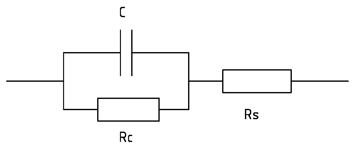
The AC measurement method, I have at this moment just tried out very momentarily. The first goal is to produce a Nyquist plot of a simple electronic setup of a resistor in series with a capacitor and a resistor, se figure 5.

Figur 5, (top) the simple electrical setup for the Nyquist measurements. (bottom) the corresponding Nyquist plot, the offset of the half cirlce from the vertical axis is related to the series resistance, while the diameter of the half circle corresponds to the capacitors parallell resistance, the height of the circle is linked to the capacitance.

I conducted this test by introducing white noise into the setup and thereafter Fourier transform the measured result to produce the Nyquist plot, as seen in figure 5. This approach is easier and quicker than the regular sweeping of the frequency method, especially if you can do it in software. 

The produced Nyquist plot shows the right shape for the electrical setup being tested but unfortunately it is not correct to the values and at least 30% error can be observed. Later I will try the more basic frequency sweeping method instead.

Conclusion
This homemade potentiostat seems to work partly, cause it shows some basic cyclic voltammetry results, however there still remains some unsolved question regarding peaks and noise as seen in the plots. The AC methods have not been tested yet to any larger extent.


There is now an update to this post in the home-made-cyclic-voltammetry-system, part II post.

Plot of resistance as function of melted particles

This is a plot of the sintering process, resistance as function of melted particles.
The resistance is shown to go up during the process. It's hard to say anything more about the behavior of the system. But at least due to the resistance increase, some of the current appears to go through the particles, not to surprising perhaps. The final resistance is on the other hand quite low meaning that good conduction still exist after the particles melted away.

Pre-phase sintering plots...

Details on the sintering process of the nano particles

I have now made some detailed plots on the observed current-jump that occurs when the nano particles fuses together. This was observed for seven of the eight experiments.

In the box archive I have put a data table for the results on the electrical properties. The samples don't have so well defined geometry, but at least they can be aranged unde some basic shapes as wire-, cluster- and grape-shaped. In three cases the need power to sinter the particles was below 1~uW, two cases at 5.9uW and 7.1uW and another two cases at 23.5uW and 34.2uW which is the highest value of them all.